Written Corrective Feedback: A Bayesian Meta-Analysis
Webpage created and maintained by Author © 2020-present
Authors
XXX University——(all authors contributed equally.)
1 Introduction
The following document includes the descriptive Bayesian meta-analysis result for Written Corrective Feedback (WCF) project.
While for this type of data, regression-based models can better account for complexity of the data structure, those models don’t produce descriptive results which are commonly reported in the field.
The following include both tables and results. These results are based on the moderators that we agreed in August 2020, and XXXX implemented all of them via programming.
The 15 refined and agreed upon moderators include:
##  [1] "setting"     "cf.type"     "error.key"   "error.type"  "ed.level"
##  [6] "profic"      "cf.oral"     "cf.training" "cf.scope"    "Length"
## [11] "instruction" "graded"      "genre"       "cf.revision" "timed"
The very final changes to the categories included:
profic: replace 77s with 99s
cf.type: replace 15s with 99s
Length: replace 0s with 1s and replace 3s with 2s (to end up with three categories: 1 & 2 & 99)
graded: replace 88s with 99s
2 Inter-rater reliability (IRR) analyses
Following Norouzian (in press), two raters rated 12% of the total study pool. The following shows the inter-rater reliability results.
| Sindex | lower | upper | conf.level | row.comprd | min.cat | n.coder | study.level |
|---|---|---|---|---|---|---|---|
| 0.63 | 0.44 | 0.78 | 0.95 | 43 | 4 | 2 | No |
| 1.00 | 1.00 | 1.00 | 0.95 | 43 | – | 2 | No |
| 0.58 | 0.35 | 0.81 | 0.95 | 43 | 1 | 2 | No |
| 0.78 | 0.33 | 1.00 | 0.95 | 6 | 1 | 2 | Yes |
| 0.95 | 0.86 | 1.00 | 0.95 | 43 | 2 | 2 | No |
| 0.75 | 0.25 | 1.00 | 0.95 | 6 | 0 | 2 | Yes |
| 1.00 | 1.00 | 1.00 | 0.95 | 6 | – | 2 | Yes |
| 0.88 | 0.77 | 0.97 | 0.95 | 43 | 0 | 2 | No |
| 1.00 | 1.00 | 1.00 | 0.95 | 6 | – | 2 | Yes |
| 0.56 | 0.11 | 1.00 | 0.95 | 6 | 0 | 2 | Yes |
| 0.94 | 0.84 | 1.00 | 0.95 | 43 | 1 | 2 | No |
| 1.00 | 1.00 | 1.00 | 0.95 | 6 | – | 2 | Yes |
| 0.25 | -0.25 | 0.75 | 0.95 | 6 | 1 | 2 | Yes |
| 1.00 | 1.00 | 1.00 | 0.95 | 6 | – | 2 | Yes |
| 0.67 | 0.00 | 1.00 | 0.95 | 6 | 0 | 2 | Yes |
| Sindex | lower | upper | conf.level | row.comprd | min.cat | n.coder | study.level | |
|---|---|---|---|---|---|---|---|---|
| cf.oral | 0.628 | 0.442 | 0.783 | 0.95 | 43 | 4 | 2 | No |
| cf.revision | 1.000 | 1.000 | 1.000 | 0.95 | 43 | – | 2 | No |
| cf.scope | 0.581 | 0.349 | 0.814 | 0.95 | 43 | 1 | 2 | No |
| cf.training | 0.778 | 0.333 | 1.000 | 0.95 | 6 | 1 | 2 | Yes |
| cf.type | 0.946 | 0.864 | 1.000 | 0.95 | 43 | 2 | 2 | No |
| ed.level | 0.750 | 0.250 | 1.000 | 0.95 | 6 | 0 | 2 | Yes |
| error.key | 1.000 | 1.000 | 1.000 | 0.95 | 6 | – | 2 | Yes |
| error.type | 0.884 | 0.767 | 0.971 | 0.95 | 43 | 0 | 2 | No |
| genre | 1.000 | 1.000 | 1.000 | 0.95 | 6 | – | 2 | Yes |
| graded | 0.556 | 0.111 | 1.000 | 0.95 | 6 | 0 | 2 | Yes |
| instruction | 0.938 | 0.845 | 1.000 | 0.95 | 43 | 1 | 2 | No |
| Length | 1.000 | 1.000 | 1.000 | 0.95 | 6 | – | 2 | Yes |
| profic | 0.250 | -0.250 | 0.750 | 0.95 | 6 | 1 | 2 | Yes |
| setting | 1.000 | 1.000 | 1.000 | 0.95 | 6 | – | 2 | Yes |
| timed | 0.667 | 0.000 | 1.000 | 0.95 | 6 | 0 | 2 | Yes |

The comprehensive IRR analyses above helped redefine, or merge a few categories in the our coding scheme improving the replicability of our meta-analytic data set and the subsequent results by other WCF researchers (see Norouzian, in press).
3 The methodology
3.1 The effect size: dint
We calculated a within-group Cohen’s d effect size for each study group (i.e., control and tretments) in a controlled study as:
\[ \tag{1} d_{D} = \frac{m_{post} - m_{pre}}{sd_D} \] where \(m_{post}\) and \(m_{pre}\) are a study group’s means at the pre- and post-testing occasions, and \(sd_D\) is the standard deviation of their difference. \(d_D\) has a purely algebraic relation to a corrosponding paired t-value targeting the same comparison:
\[ \tag{2} d_{D} = \frac{t_{paired}}{\sqrt{n}} \]
where \(n\) is the number of a study group’s participants. As a result, in several studies (e.g., Jhowry, 2010; Mubarak, 2013) that had reported paired t-values, \(d_D\) was directly recovered for the relavant study group.
In other cases where only \(sd_D\) was instead reported (e.g., Karim & Nassaji, 2014; Nakazawa, 2006), equation (1) was used to obtain \(d_D\). Finally, in cases where neither \(t_{paired}\) nor \(sd_D\) for a study group’s change between the two testing occasions were reported, we obtained \(sd_D\) using one of the following methods: (a) by imputation using a pre-post correlation (\(r_D\)) obtainable from another group in the same study or (b) assuming a medium-high correlation (\(r_D = .6\)) following the recommendations by Ray and Shadish (1996) and Viechtbauer (2007) for the missing correlation and then using it in:
\[ \tag{3} sd_D =\sqrt{sd_{pre}^2+sd_{post}^2-2(r_D)sd_{pre}sd_{post}} \]
Once \(sd_D\) was obtained, then \(d_{D}\) using equation (1) was calculated.
It is well-known that \(d_{D}\) is a biased estimator of its real population value (Becker, 1988; Morris, 2000; Morris & DeShon, 2002; Viechtbauer, 2007). Therefore, to address the bias, we used Hedges’ (1981) correction factor (\(cf\)):
\[ \tag{4} cf = \frac{\Gamma\bigg(\frac{df}{2}\bigg)}{\sqrt{\frac{df}{2}} \Gamma\bigg(\frac{df-1}{2}\bigg)} \approx 1- \frac{3}{4df-1} \] where \(\Gamma\) is a mathemtical function available in many software programs (e.g., R or Excel) and \(df\) is simply \(n-1\). The equation after the \(\approx\) sign is an approximation for the exact correction factor. In our study, the bias-corrected effect size, \(g_{D}\), was computed as:
\[ \tag{5} g_{D} = cf \times d_{D} \]
The unbiased estimator of the sampling variance, \(V(g_{D})\), was computed (see Viechtbauer, 2007; equation 26) as: \[ \tag{6} V(g_{D}) = \frac{1}{n} + \bigg(1-\frac{df-2}{df\times cf^2}\bigg)\times g_{D}^2 \]
Once the unbiased estimate of effect size (\(g_{D}\)) and its unbiased sampling variance (\(V(g_{D})\)) for each pair of treatment and control groups were obtained, we then calculated their difference (see Morris & DeShon, 2002) to which we refer as a \(dint\):
\[ \tag{7} dint = g_{D_T} - g_{D_C} \] where the \({_T}\) and \({_C}\) subscripts denote the treatment and the control groups, respectively. The unbiased sampling variance of a \(dint\) is computed as:
\[ \tag{8} V(dint) = V(g_{D_T}) + V(g_{D_C}) \]
3.2 Why this effect size
This effect size, we believe, closely matches the study designs in the WCF literature which often follow a nonequivalent groups design (NEGD) shown as:
N O X O O
N O – O O
where \(N\) is non-random assignment of participants, \(O\) is an observation collected at a testing occasion, and \(X\) is a form of WCF (i.e., treatment).
Given this design, a \(dint\) measures the change within a treatment group across any two times (e.g., pre- to immediate post-test) and compares it to that within the control group. For example, a \(dint\) of \(+0.2\) for a WCF treatment would indicate that the treatment group’s standardized mean change is \(+0.2\) higher than that of the control group in the time period considered (e.g., pre- to immediate post-test).
Therefore, \(dint\) can be thought of as measuring the simple-effect of study group membership (e.g., treatment vs. control) at each time interval in the primary studies. We believe this effect size is suited to the longitudinal but also casual aspects of WCF studies. This is because measuring a \(dint\) is also equivalent to measuring difference in differences (DID), an approach known to mitigate some extraneous factors and selection biases arising from non-random assignment of study participants to the study groups (Angrist & Pischke, 2008).
3.3 Handling dependency among effect sizes
We included all complex-structure WCF studies including multi-outcome, multi-group, and multiple-posttest studies. This stage led to 524 within-group Cohen’s d effect sizes, and 262 dints. Adopting an open-science approach, our full dataset for this study is publicly available HERE (this is another new, updated shortened dataset for this publication only).
20 of the total 52 studies contained one or more negative dints before averaging multiple \(dints\) in each study. The unbiased sampling variance of the averaged \(dint\) in each study, \(V(\frac{1}{m}\sum_{i=1}^m dint_i)\), was computed using (see Borenstein, et al., 2009, Chapter 24):
\[ \tag{9} V\bigg(\frac{1}{m}\sum_{i=1}^m dint_i \bigg) = \bigg(\frac{1}{m}\bigg)^2 \times\bigg(\sum_{i=1}^m V_i+\sum_{i\neq j} (r_{ij} \times \sqrt{V_i} \times \sqrt{V_j} ) \bigg) \] where \(m\) is the number of \(dints\) in each study, \(r_{ij}\) denotes the assumed correlation between any two \(dints\) from the same study (we asummed \(r_{ij}\) = .5), and \(V_i\) and \(V_j\) are their individual unbiased sampling variances as obtained in equation 8.
Eight average effect sizes from 8 studies (i.e., Bitc_Yng_Cmrn; Diab_b; Eki_diGnro; Fazio; Jhowry; Trscott_Hsu; VanBe_Jng_Ken; Zhang) became negative. See the Outlier control and publication bias section for a discussion of how outlying effect sizes were treated.
4 Meta-analysis model
The model of our meta-analysis study is Bayesian random-effects designed to estimates 2 parameters which are diagrammatically shown in the following Figure:
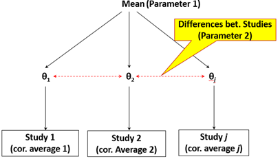
In the above figure, parameter 1 is the mean (\(\mu\)) or overall effect size, and parameter 2 is Tau (\(\tau\)) or standard deviation of the distribution of the study effect sizes.
As explained in Norouzian et al., (2018, 2019), in Bayesian inference, all parameters of a model (e.g., \(\mu\), and \(\tau\)) are estimated such that a direct statement about their population values can be conveyed to the research audience.
This is possible because Bayesian meta-analyses provide a range of credible estimates of the true mean effect (\(\mu\)) of effect sizes, their standard deviation (\(\tau\)) based on the individual effect sizes and sampling variances of effect sizes fit to it. Thus, for each meta-analytic parameter, we often speak of a (marginal) posterior distribution which may be described using familar summary statistics (e.g., mean, sd etc.) as well as Highest Density Intervals (HDI) that cover 95% of it (see Norouzian et al., (2018, 2019) for more details).
5 Outlying effect sizes
Following the outlier detection method of removing the effect sizes that fall beyond \(\pm 3\) standard deviations from their mean (Lipsey & Wilson, 2001), five effect sizes were eliminated from the dataset as shown below:
| study.name | row | dint |
|---|---|---|
| Nemati_etal | 152 | 5.093062 |
| Nemati_etal | 150 | 4.613584 |
| Al_Ajmi | 6 | 4.376457 |
| Seiff_ElSak | 186 | 4.009361 |
| Al_Ajmi | 5 | 3.444227 |
Removal of the above effect sizes led to the removal of the following studies:
## [1] "Al_Ajmi" "Seiff_ElSak"The positively skewed distribution of our effect sizes before and the symmetric distribution of effect sizes after the ouliers’ removal is captured in the figures below.


As noted earlier, a number of effect sizes were also negative. The full list of these effect sizes is as follows:
| study.name | dint | SD |
|---|---|---|
| Al.Ahm_Al.Jar | -0.1553864 | 0.4272827 |
| Bitc_Yng_Cmrn | -0.4935793 | 0.3802870 |
| Bitc_Yng_Cmrn | -0.5156586 | 0.3467887 |
| Bitc_Yng_Cmrn | -0.6975506 | 0.3574931 |
| Brown | -0.1324652 | 0.2208191 |
| Brown | -0.2091514 | 0.2219060 |
| Diab_b | -0.0241685 | 0.3318732 |
| Diab_b | -0.6605675 | 0.3429860 |
| Eki_diGnro | -0.5477378 | 0.3487669 |
| Eki_diGnro | -0.2352528 | 0.3435118 |
| Elis_Sh_Mur_Tak | -0.0130216 | 0.4873301 |
| Fazio | -0.1308920 | 0.3642787 |
| Fazio | -0.5467906 | 0.3915234 |
| Hartshorn | -0.2508190 | 0.2994754 |
| Jhowry | -0.0618444 | 0.4750960 |
| Karim_End. | -0.3485250 | 0.3275155 |
| Karim_End. | -0.2824068 | 0.3230654 |
| Mubarak | -0.1189049 | 0.4172375 |
| Mubarak | -0.0883446 | 0.3988416 |
| Mubarak | -0.4926680 | 0.4258486 |
| Mubarak | -1.3695479 | 0.5306183 |
| Mubarak | -0.1587712 | 0.3887653 |
| Mubarak | -0.3610557 | 0.4024929 |
| Munoz | -0.1428038 | 0.3358399 |
| Nusrat.etal. | -0.2210411 | 0.2840090 |
| Nusrat.etal. | -0.1870419 | 0.2983482 |
| Parreno | -0.2291886 | 0.3701226 |
| Pash. | -0.0758471 | 0.3323983 |
| Sheen_etal | -0.3736234 | 0.3363308 |
| Sheen_etal | -0.1539893 | 0.3416138 |
| Sheen_etal | -1.1416347 | 0.5460815 |
| Sheen_etal | -0.9534229 | 0.5584261 |
| Sheen_etal | -0.6841150 | 0.4297241 |
| Sheen_etal | -0.6391715 | 0.5002314 |
| Sheen_etal | -0.7079216 | 0.4999521 |
| Stefan_Revesz | -0.4877348 | 0.2737911 |
| Stefan_Revesz | -0.1259811 | 0.2674519 |
| Trscott_Hsu | -0.0827458 | 0.3412078 |
| VanBe_Jng_Ken | -0.8911023 | 0.3758384 |
| VanBe_Jng_Ken | -1.3161183 | 0.4266433 |
| VanBe_Jng_Ken | -0.1756171 | 0.4101802 |
| VanBe_Jng_Ken | -1.0457147 | 0.3657065 |
| VanBe_Jng_Ken | -0.2850271 | 0.3514128 |
| VanBe_Jng_Ken | -0.7674492 | 0.3761727 |
| VanBe_Jng_Ken | -0.0067616 | 0.3622921 |
| VanBe_Jng_KenB | -0.0583938 | 0.2515945 |
| VanBe_Jng_KenB | -0.0023592 | 0.2552378 |
| Zhang | -0.8209664 | 0.3198808 |
| Zhang | -0.7342465 | 0.3112923 |
5.1 Outlier control
From our initial 52 studies, two studies (Al_Ajmi and Seiff_ElSak) were excluded because (a) they included extremely large effect sizes (e.g., 5.09) that had extreme effect on the overall effect, (b) a close inspection of the studies’ treatments, settings, operational definitions and detailed procedures did not suggest any notable difference to justify such drastically large effects relative to other studies in the WCF literature and (c) they made the funnel plot of the study effect sizes extremely asymmetric causing the egger’s test of funnel plot symmetry to become highly significant (p < .001).
|
For the sake of transparency, our dataset before the treatment of outlying effect sizes is publicly available HERE and our dataset after the treatment of outlying effect sizes is also publicly available HERE.
6 Publication bias
6.1 Funnel plot
After the treatment of the outlying effect sizes as described in the previous section, our first method of detecting publication bias was a visual funnel plot. In the funnel plot below, while not perfectly symmetrical, average effects sizes from each study appear to be moderately symmetrical on both sides of the overall mean effect (the middle dasshed line). It is worth noting that the gray points in the plot are the shrinkage estimates i.e., more exreme (in absolute value) and less precise (those with larger SE) effect sizes are shrunk more toward the mean effect via random-effects model and Bayesian shrinkage i.e., use of a prior on the mean effect size to blunt extreme effect sizes from studies.

Because, the detection of publication bias via a funnel plot is mainly a visual method, it may sometimes turn out to be subjective. As a result, we used several other statistical methods to examine publication bias in the WCF literature.
6.2 Egger’s Test
We also conducted an Egger’s test (Egger, Smith, Schneider, & Minder, 1997) of funnel plot symmetry. Using this test, we examined the extent to which the standard error (i.e., precision) of the effect sizes collected from the WCF literature related to the effect sizes’ magnitude. If such a relationship rises to a statistically significant level, that could suggest publication bias and asymmetry in the funnel plot of effect sizes.
In our case, given that the p-value for the egger’s test was larger than .05, we concluded that our funnel plot is symmetric and the likelihood of publication bias in the collected sample of WCF studies is small.
|
6.3 Trim and Fill Method
We also assessed the risk of pubication bias via a third method known as Trim and Fill (Duval, 2005; Duval & Tweedie, 2000). In this non-parameteric method, the goal is to impute (i.e., fill) the possible effect sizes missing, due to a particular selection mechanism, from the literature to achieve a more symmetric funnel plot of effect sizes on either side of the plot.
As shown in the follwing figure, in our case, the Trim and Fill method suggested that no fill-studies to either side of the plot are needed to achieve a more symteric view of the WCF literature. Therefore, these results concur with with the previous egger’s test result as regards the issue of publication bias.

6.4 Vevea and Hedges Method
We also used a fourth confirmatory method to detect publication bias. Vevea and Hedges (1995) proposed a method where the original meta-analysis and a bias-assumed meta-analysis using weights associated with the p-value intervals for effect sizes are compared to one another (see Vevea & Hedges 1995 and Vevea & Woods, 2005 for details).
Once both the original and bias-assumed meta-analytic models are obtained, a likelihood-ratio test compares the fit of the two models to the effect sizes. A statistically significant likelihood-ratio test would indicate that the bias-assumed model better fits the study effect sizes, and hence the presence of publication bias. Otherwise, the risk of publicatio bias is minimal.
| Df | X^2 | p.value | |
|---|---|---|---|
| Likelihood Ratio Test: | 1 | 0.1079 | 0.7426 |
6.5 Orwin’s Fail-safe N method
Finally, we conducted the Orwin’s (1983) Fail-safe N method. Using this method, we examined the number of missing WCF studies needed to decrease our meta-analytic WCF effect to the point of triviality. We set the triviality of our meta-analytic effect to be \(0.05\).
The likelihood of publication bias increases, if only a handful of studies would be needed to deem our meta-analytic effect trivial. This is because it is possible that a handful of small-effect studies might not have made their way into the published WCF literature. Conversely, the likelihood of publication bias decreases, if a relatively large number of studies would be needed to deem our meta-analytic effect trivial. This is because it is less likely that such a large number of small-effect studies constituting a trend in a domain of research might not have made their way into the published WCF literature.
| studies.needed.to.tiviality | trivial.effect.size |
|---|---|
| 478 | 0.05 |
Once again, based on the relatively large number of missing studies suggested by the Fail-safe N Method to deem our meta-analytic effect trivial, the likelihood of publication bias seems to be low.
As can be seen, the methods of publication bias often complement each other each viweing bias from a unique perspective. But overall, our visual (funnel plot), and statistical methods (Egger’s test, Trim and Fill, Vevea and Hedges’ test, and Orwin’s Fail-safe N) collectively suggested no major indication of publication bias in the present pool of studies.
7 The Effect of WCF
7.1 Definition of tabular output
In the following tables, Mu denotes the posterior mean for the mean effect in a Bayesian random-effects meta-analysis conducted in each row of the table.
In the following tables, Low and Up denote the 95% Bayesian high-density credible intervals for the posterior mean effect. They give us an indication of the 95% most credible effect sizes had we collected the entire population of WCF studies ever conducted.
In the following tables, Perc.mu denotes the percentage interpretation of the mean effect in each row of the table. Any percentage larger than 0% shows an improvement for treatment groups over control groups in the WCF literature in each row of the table
In the following tables, K denotes the number of studies. However, because a single study could possess group-level features (e.g., some groups receiving oral feedback, but not others), it may be counted multiply in the K column. Therefore, the K column total could be larger than 50, the total number of studies, for group-level moderators. For study-level moderators (e.g., proficiency), K column total always equals 50.
In the following tables, BF01.mu denotes a Bayes Factor (see Norouzian et al, 2019). It tells us if the mean effect in each row of the table could provide evidence in favor of the null hypothesis that mean effect = 0. The smaller the value, the larger the evidence against the null hypothesis (and in favor of the alternative hypothesis i.e., mean effect \(\neq\) 0).
In the following tables, BF01.tau denotes a Bayes Factor (see Norouzian et al, 2019). It tells us if the heterogeneity between studies’ mean effects (\(\tau\)) in each row of the table could provide evidence in favor of the null hypothesis that heterogeneity = 0. The smaller the value, the larger the evidence against the null hypothesis (and in favor of the alternative hypothesis i.e., heterogeneity \(\neq\) 0).
Closely related to tau (heterogeneity in effect sizes in sd unit), is I2 (Higgins and Thompson 2002; Higgins, Thompson, Deeks, & Altman, 2003). I2 denotes the percentage of the total variability in a set of effect sizes due to between-study heterogeneity. Higgins and Thompson (2002) proposed a tentative classification of I2 values where percentages of around 25% (I2 = 25), 50% (I2 = 50), and 75% (I2 = 75) would denote low, medium, and high heterogeneity, respectively.
7.2 WCF Overall Effect (disregarding time)

7.3 Overall effectiveness (with time to posttest)

| code | K | mu | low | up | I2 | tau | BF01.mu | BF01.tau | perc.mu |
|---|---|---|---|---|---|---|---|---|---|
| time.1 | 22 | 0.7143 | 0.5296 | 0.8986 | 0.4219 | 0.2653 | 0 | 0.8955 | 26.25% |
| time.2 | 25 | 0.4645 | 0.2076 | 0.7245 | 0.813 | 0.5537 | 0.0558 | 0 | 17.89% |
| time.3 | 20 | 0.5586 | 0.2647 | 0.857 | 0.7938 | 0.5568 | 0.0372 | 1e-04 | 21.18% |
| time.4 | 12 | 0.4744 | 0.1574 | 0.7905 | 0.6359 | 0.4034 | 0.2625 | 0.1546 | 18.24% |
| code | K | mu | low | up | I2 | tau | BF01.mu | BF01.tau | perc.mu | |
|---|---|---|---|---|---|---|---|---|---|---|
| immediate | time.1 | 22 | 0.7143 | 0.5296 | 0.8986 | 0.4219 | 0.2653 | 0 | 0.8955 | 26.25% |
| short | time.2 | 25 | 0.4645 | 0.2076 | 0.7245 | 0.813 | 0.5537 | 0.0558 | 0 | 17.89% |
| medium | time.3 | 20 | 0.5586 | 0.2647 | 0.857 | 0.7938 | 0.5568 | 0.0372 | 1e-04 | 21.18% |
| long | time.4 | 12 | 0.4744 | 0.1574 | 0.7905 | 0.6359 | 0.4034 | 0.2625 | 0.1546 | 18.24% |
7.4 Setting

| K | mu | low | up | I2 | tau | BF01.mu | BF01.tau | perc.mu | |
|---|---|---|---|---|---|---|---|---|---|
| SL | 16 | 0.4528 | 0.195 | 0.7143 | 0.6183 | 0.3805 | 0.0957 | 0.1268 | 17.47% |
| FL | 34 | 0.5276 | 0.3331 | 0.7234 | 0.773 | 0.4819 | 4e-04 | 0 | 20.11% |
| lower | upper | diff. | |
|---|---|---|---|
| SL vs FL | -0.3963687 | 0.2504415 | FALSE |
7.5 Educational level

| K | mu | low | up | I2 | tau | BF01.mu | BF01.tau | perc.mu | |
|---|---|---|---|---|---|---|---|---|---|
| high School | 6 | 0.5128 | -0.1536 | 1.1917 | 0.8749 | 0.6623 | 1.5846 | 0.0113 | 19.6% |
| university | 39 | 0.4871 | 0.345 | 0.6299 | 0.6011 | 0.3318 | 0 | 4e-04 | 18.69% |
| institute | 4 | 0.8757 | -0.3399 | 2.0819 | 0.9096 | 1.0696 | 1.0695 | 0 | 30.94% |
| lower | upper | diff. | |
|---|---|---|---|
| high School vs university | -0.6534242 | 0.7182970 | FALSE |
| high School vs institute | -1.7192808 | 1.0267806 | FALSE |
| university vs institute | -1.5898565 | 0.8506671 | FALSE |
7.6 Proficiency

| K | mu | low | up | I2 | tau | BF01.mu | BF01.tau | perc.mu | |
|---|---|---|---|---|---|---|---|---|---|
| beginner | 3 | 0.9819 | -0.4869 | 2.4201 | 0.9091 | 1.1294 | 1.021 | 2e-04 | 33.69% |
| advanced | 32 | 0.5172 | 0.3378 | 0.6975 | 0.7027 | 0.409 | 2e-04 | 0 | 19.75% |
| intermediate | 6 | 0.5789 | 0.1947 | 0.9651 | 0.2464 | 0.1967 | 0.2262 | 3.5024 | 21.87% |
| mixed/not reported | 9 | 0.2711 | -0.0622 | 0.5974 | 0.6705 | 0.3521 | 2.8172 | 0.5472 | 10.68% |
| lower | upper | diff. | |
|---|---|---|---|
| beginner vs advanced | -1.0403291 | 1.8880292 | FALSE |
| beginner vs intermediate | -1.1362802 | 1.8650883 | FALSE |
| beginner vs mixed/not reported | -0.8149559 | 2.1581149 | FALSE |
| advanced vs intermediate | -0.4859261 | 0.3631019 | FALSE |
| advanced vs mixed/not reported | -0.1222468 | 0.6236818 | FALSE |
| intermediate vs mixed/not reported | -0.1959408 | 0.8161790 | FALSE |
7.7 WCF Type

| K | mu | low | up | I2 | tau | BF01.mu | BF01.tau | perc.mu | |
|---|---|---|---|---|---|---|---|---|---|
| direct | 29 | 0.4479 | 0.2329 | 0.6627 | 0.744 | 0.4827 | 0.0154 | 0 | 17.29% |
| location | 16 | 0.5277 | 0.1365 | 0.9176 | 0.8466 | 0.6769 | 0.378 | 0 | 20.11% |
| error coding | 17 | 0.4804 | 0.2815 | 0.6895 | 0.4709 | 0.2603 | 0.004 | 0.7905 | 18.45% |
| metalinguistic | 9 | 0.4953 | 0.0978 | 0.9133 | 0.6274 | 0.4269 | 0.4983 | 0.3534 | 18.98% |
| direct+metalinguistic | 13 | 0.7206 | 0.4038 | 1.0454 | 0.6695 | 0.4318 | 0.0113 | 0.1214 | 26.44% |
| other | 2 | 0.1971 | -0.863 | 1.2455 | 0.5253 | 0.3791 | 5.2457 | 1.9406 | 7.81% |
7.8 Scope

| K | mu | low | up | I2 | tau | BF01.mu | BF01.tau | perc.mu | |
|---|---|---|---|---|---|---|---|---|---|
| unfocused | 19 | 0.3448 | 0.1006 | 0.5903 | 0.6738 | 0.4118 | 0.4337 | 0.0026 | 13.49% |
| mid-focused | 12 | 0.3478 | 0.0941 | 0.6117 | 0.5842 | 0.2926 | 0.5068 | 1.2041 | 13.6% |
| focused | 23 | 0.6979 | 0.4569 | 0.9402 | 0.7114 | 0.4669 | 3e-04 | 7e-04 | 25.74% |
7.9 Error Type

| K | mu | low | up | I2 | tau | BF01.mu | BF01.tau | perc.mu | |
|---|---|---|---|---|---|---|---|---|---|
| mixed | 26 | 0.3013 | 0.1145 | 0.4873 | 0.6331 | 0.3571 | 0.2287 | 0.0045 | 11.84% |
| articles | 16 | 0.5772 | 0.3361 | 0.8214 | 0.6535 | 0.3673 | 0.0063 | 0.0262 | 21.81% |
| prepositions | 5 | 0.5581 | -0.1285 | 1.2307 | 0.7994 | 0.571 | 1.2586 | 0.0787 | 21.16% |
| verb tense | 5 | 0.86 | -0.2769 | 1.988 | 0.9152 | 1.1417 | 1.0677 | 0 | 30.51% |
| other | 6 | 0.4233 | -0.1065 | 1.0127 | 0.734 | 0.4699 | 1.6878 | 0.7215 | 16.4% |
7.10 Key

| K | mu | low | up | I2 | tau | BF01.mu | BF01.tau | perc.mu | |
|---|---|---|---|---|---|---|---|---|---|
| no key | 4 | 0.4068 | -0.1669 | 1.0319 | 0.4737 | 0.3078 | 2.028 | 2.0862 | 15.79% |
| key provided | 16 | 0.4665 | 0.2652 | 0.6771 | 0.4705 | 0.2553 | 0.0086 | 0.9161 | 17.96% |
| N/A | 40 | 0.5026 | 0.3016 | 0.704 | 0.8121 | 0.5586 | 0.001 | 0 | 19.24% |
| lower | upper | diff. | |
|---|---|---|---|
| No key vs key provided | -0.6592533 | 0.6011986 | FALSE |
| No key vs NA | -0.6918739 | 0.5648004 | FALSE |
| key provided vs NA | -0.3184139 | 0.2562545 | FALSE |
7.11 Revision

| K | mu | low | up | I2 | tau | BF01.mu | BF01.tau | perc.mu | |
|---|---|---|---|---|---|---|---|---|---|
| not required | 6 | 0.6749 | 0.2274 | 1.1468 | 0.5973 | 0.3468 | 0.1983 | 1.3845 | 25.01% |
| required | 31 | 0.4863 | 0.307 | 0.6685 | 0.6838 | 0.3924 | 5e-04 | 0.0032 | 18.66% |
| feedback reviwed | 9 | 0.427 | -0.0982 | 0.9533 | 0.8305 | 0.6585 | 1.9778 | 0 | 16.53% |
| not reported | 5 | 0.4685 | -0.2003 | 1.1203 | 0.8185 | 0.5612 | 1.8635 | 0.0337 | 18.03% |
7.12 Oral supplemental CF

| K | mu | low | up | I2 | tau | BF01.mu | BF01.tau | perc.mu | |
|---|---|---|---|---|---|---|---|---|---|
| not provided | 50 | 0.494 | 0.3408 | 0.6479 | 0.7349 | 0.4523 | 0 | 0 | 18.93% |
| provided | 5 | 0.7662 | 0.0558 | 1.5169 | 0.712 | 0.5723 | 0.4869 | 0.5217 | 27.82% |
7.13 Genre

| K | mu | low | up | I2 | tau | BF01.mu | BF01.tau | perc.mu | |
|---|---|---|---|---|---|---|---|---|---|
| academic | 16 | 0.3712 | 0.0974 | 0.6461 | 0.7389 | 0.4372 | 0.5088 | 0.0021 | 14.48% |
| visual description | 19 | 0.6341 | 0.4117 | 0.8574 | 0.5642 | 0.3454 | 8e-04 | 0.1541 | 23.7% |
| narrative/journal | 9 | 0.3778 | 0.0486 | 0.7038 | 0.5864 | 0.3323 | 0.9299 | 0.6502 | 14.72% |
| reading summary | 2 | 0.6306 | -0.5663 | 1.7672 | 0.815 | 0.5276 | 1.3293 | 0.9064 | 23.58% |
| not reported | 3 | 0.8049 | -0.7244 | 2.3157 | 0.935 | 1.2202 | 1.5145 | 0 | 28.96% |
| lower | upper | diff. | |
|---|---|---|---|
| academic vs visual description | -0.6143674 | 0.0890175 | FALSE |
| academic vs narrative/journal | -0.4286789 | 0.4201417 | FALSE |
| academic vs reading summary | -1.3964923 | 0.9867740 | FALSE |
| academic vs not reported | -1.9497568 | 1.1388604 | FALSE |
| visual description vs narrative/journal | -0.1347535 | 0.6523789 | FALSE |
| visual description vs reading summary | -1.1250137 | 1.2422710 | FALSE |
| visual description vs not reported | -1.6792161 | 1.3946423 | FALSE |
| narrative/journal vs reading summary | -1.4011992 | 1.0023588 | FALSE |
| narrative/journal vs not reported | -1.9525921 | 1.1538611 | FALSE |
| reading summary vs not reported | -2.0572747 | 1.7039127 | FALSE |
7.14 Timed

| K | mu | low | up | I2 | tau | BF01.mu | BF01.tau | perc.mu | |
|---|---|---|---|---|---|---|---|---|---|
| no limit | 8 | 0.4182 | -0.0276 | 0.8643 | 0.6983 | 0.4656 | 1.4257 | 0.1171 | 16.21% |
| limited | 41 | 0.5225 | 0.3511 | 0.6951 | 0.7531 | 0.462 | 0 | 0 | 19.93% |
| lower | upper | diff. | |
|---|---|---|---|
| timed 0 vs timed 1 | -0.580076 | 0.3714433 | FALSE |
7.15 Grading

| K | mu | low | up | I2 | tau | BF01.mu | BF01.tau | perc.mu | |
|---|---|---|---|---|---|---|---|---|---|
| not graded | 20 | 0.4684 | 0.284 | 0.6543 | 0.5657 | 0.2908 | 0.0033 | 0.1714 | 18.03% |
| graded | 10 | 0.2554 | -0.0928 | 0.6008 | 0.7759 | 0.4317 | 3.7852 | 0.0217 | 10.08% |
| not reported | 21 | 0.6656 | 0.3703 | 0.963 | 0.7695 | 0.5722 | 0.0065 | 0 | 24.72% |
| lower | upper | diff. | |
|---|---|---|---|
| not graded vs graded | -0.1756498 | 0.6066272 | FALSE |
| not graded vs not reported | -0.5466881 | 0.1499102 | FALSE |
| graded vs not reported | -0.8660679 | 0.0404682 | FALSE |
7.16 Length of writing

| K | mu | low | up | I2 | tau | BF01.mu | BF01.tau | perc.mu | |
|---|---|---|---|---|---|---|---|---|---|
| short | 17 | 0.5076 | 0.3056 | 0.7073 | 0.5596 | 0.2902 | 0.0057 | 0.3134 | 19.41% |
| long | 12 | 0.3111 | -0.0215 | 0.6436 | 0.7136 | 0.4455 | 2.1368 | 0.0073 | 12.21% |
| not reported | 21 | 0.6315 | 0.3325 | 0.9347 | 0.813 | 0.5908 | 0.0115 | 0 | 23.61% |
| lower | upper | diff. | |
|---|---|---|---|
| short vs long | -0.1908825 | 0.5827446 | FALSE |
| short vs not reported | -0.4888517 | 0.2325511 | FALSE |
| long vs not reported | -0.7693140 | 0.1235888 | FALSE |
7.17 Instruction on grammar

| K | mu | low | up | I2 | tau | BF01.mu | BF01.tau | perc.mu | |
|---|---|---|---|---|---|---|---|---|---|
| no instruction | 22 | 0.5924 | 0.3439 | 0.8434 | 0.8046 | 0.495 | 0.0042 | 0 | 22.32% |
| targeted instruction | 10 | 0.5004 | 0.1498 | 0.8857 | 0.6035 | 0.387 | 0.2585 | 0.8404 | 19.16% |
| untargetd instruction | 3 | -0.0506 | -1.1374 | 1.0305 | 0.8871 | 0.736 | 5.6187 | 0.0266 | -2.02% |
| not reported | 16 | 0.5375 | 0.2729 | 0.8023 | 0.6112 | 0.3913 | 0.0291 | 0.0789 | 20.45% |
| lower | upper | diff. | |
|---|---|---|---|
| no instruction vs targeted instruction | -0.3722645 | 0.5159173 | FALSE |
| no instruction vs untargetd instruction | -0.4628794 | 1.7539212 | FALSE |
| no instruction vs not reported | -0.3062954 | 0.4181211 | FALSE |
| targeted instruction vs untargetd instruction | -0.5800523 | 1.6935815 | FALSE |
| targeted instruction vs not reported | -0.4690977 | 0.4352727 | FALSE |
| untargetd instruction vs not reported | -1.7007655 | 0.5197469 | FALSE |
7.18 Training students in responding to feedback

| K | mu | low | up | I2 | tau | BF01.mu | BF01.tau | perc.mu | |
|---|---|---|---|---|---|---|---|---|---|
| no training | 12 | 0.7112 | 0.2238 | 1.2013 | 0.8737 | 0.7346 | 0.192 | 0 | 26.15% |
| received training | 7 | 0.4673 | 0.1892 | 0.7522 | 0.4014 | 0.2001 | 0.1751 | 2.5393 | 17.99% |
| not reported | 31 | 0.4337 | 0.2552 | 0.6132 | 0.66 | 0.3885 | 0.0022 | 2e-04 | 16.77% |
| lower | upper | diff. | |
|---|---|---|---|
| no training vs received training | -0.3185255 | 0.8061647 | FALSE |
| no training vs not reported | -0.2403194 | 0.7978463 | FALSE |
| received training vs not reported | -0.2952711 | 0.3689505 | FALSE |